Calibration curves are used to determine the concentration of a sample with an unknown concentration. Here, so-called standard solutions with similar properties to the sample to be measured are created and their absorbance is measured.
The concentration of the standard solutions is known, so that the measured absorbance can be plotted against the concentration. If the absorbance of the sample with unknown absorbance is subsequently measured, the concentration can be calculated with a simple formula.1
Learn more in this text about:
- The determination of the concentration of a substance with the help of a calibration curve
- The calibration of a spectrophotometer
- The aim of a calibration and in which laboratory situations it is used
- The advantages of the fluidlab R-300 when creating calibration curves
Test the fluidlab R-300 free of charge and without obligation!
You would like to make your daily laboratory routine even more efficient or carry out analyses independent of location and are interested in innovative technology that aims to do just that? Then test our patented fluidlab R-300 now - without any obligation!
Request test device now
With the aid of a calibration curve, the concentration of a substance can be determined
Calibration curves are used in analytical chemistry as a general method to determine the unknown concentration of a substance in a sample (analyte). The determination is made by comparing the sample with a series of standard samples whose concentrations are known.
The concentration of the substance to be measured leads to a change in the analytical signal or instrumental response, which can be indicated by a calibration curve.
In most cases, a linear relationship results when ordering the instrument response against the concentration of the standards.1
What are the requirements for the standard samples?
It is important to select a suitable standard sample for calibration in order to be able to calculate the concentration of the analyte.
Therefore, the selected reference should meet the following requirements:2
- same matrix as analyte
- very small systematic errors (e.g. volatilization, volume errors, etc.)
- high reproducibility
How does the calibration of a spectrophotometer work?
In general, calibration is the checking of measuring instruments whose specifications are not regulated by law. The calibration of measuring instruments is important because it guarantees, for example, quality assurance or compliance with process regulations, such as DIN EN ISO 9001:2000.3
With the help of a calibration, the relationship between the measured values or the expectation of the output variable and the true value of the input variable present measured variable for the measuring device under consideration can be determined under specified conditions.4
UV/Vis measurement with spectrophotometers is used particularly frequently in clinical chemistry, the pharmaceutical industry, research or also in quality assurance. There are regulations that require a regular performance check of the spectrophotometers used.5
The calibration of the spectrophotometer is performed with specially designed optical filters. These have certain absorption characteristics and exhibit an absorption maximum at certain wavelengths. The absorbance of each filter is measured in turn. This ranges from low to high and is therefore determined in a wide absorbance range of approx. 0.3-2. The absorbance values obtained are then compared with the nominal values of the filters. The deviation should not be more than 1%.5
Calibration curve for calculation of the concentration content
If the photometer is calibrated correctly, measurements can be performed on it. Before measuring a sample with an unknown concentration (analyte), a calibration curve is created. This is done by creating standard solutions with different concentrations. If the concentration of a protein is measured, BSA (Bovine Serum Albumin) is often used as a standard sample.
It is important that the initial concentration of the reference is known. This is then diluted so that 3-10 (Fig.1 (Ref 1- 5)) samples with different concentrations are prepared. These are measured on the photometer and the absorbance of each sample is noted.
Next, the measured absorbance is plotted against the concentration of the dilution (Fig. 1). This results in the calibration curve and a corresponding equation.5
After the calibration curve has been created by means of a dilution series of the standard solution, the concentration of an analyte (Fig.1 (sample with unknown concentration)) in a sample can now be determined. The measured concentration should be in the range of the dilutions, i.e. between the lowest and highest concentration of the standard solution (Fig.1). If this is not the case, the standard must be further diluted or concentrated and the measurements carried out again. This is done until the absorbance value of the analyte is on the calibration curve.
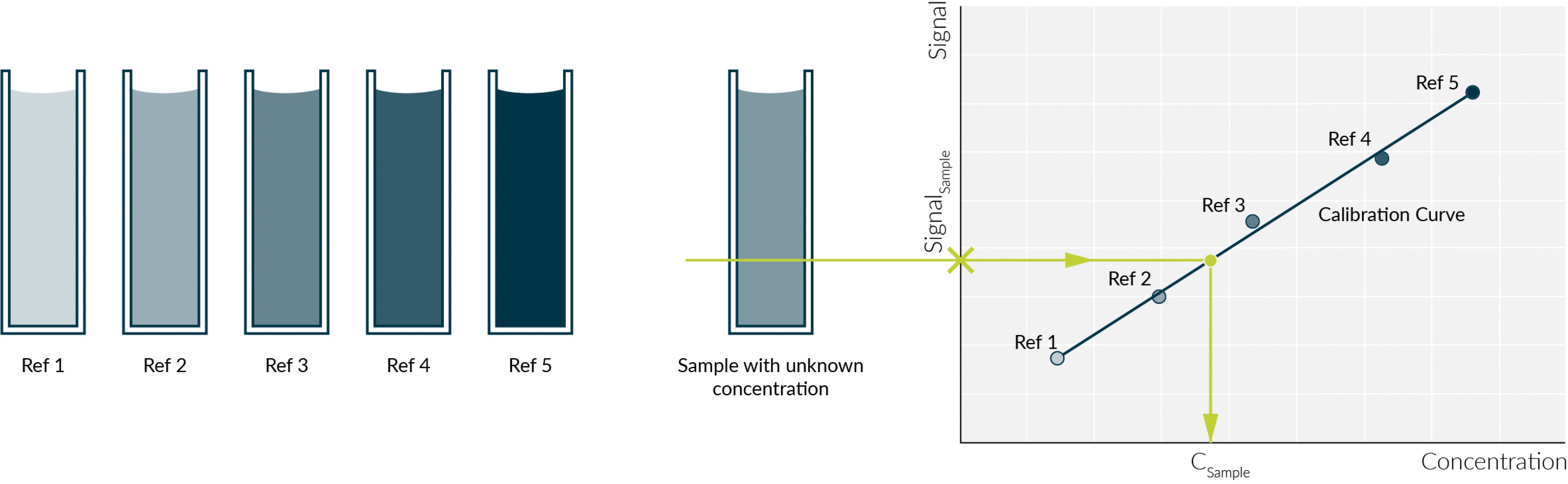
Fig. 1 A standard solution was diluted (Ref 1- Ref 5) and its absorbance was measured to create a calibration curve (right). The calibration curve can then be used to determine the concentration of the unknown sample
From the calibration curve obtained, an associated equation is obtained. Subsequently, the absorbance value of the analyte to be examined can be entered into this formula and converted to the concentration and calculated.
Are all calibration curves linear?
Calibration curves do not always run linearly. This happens when the signals obtained do not follow the concentration linearly over the entire measuring range. In these cases, the absolute term (b0) of the calibration function may be particularly large. If a small range is not linear, a linear fit can be performed without leading to large errors (Fig. 3). However, if the range is exceeded, errors may occur. Therefore, for nonlinear calibration curves, adjustments of the nonlinear functions should be performed.5

Fig. 3 In a small linear range, this can be used for concentration determination. The linear range should not be left. A: 1st measurement, B: 2nd measurement, b0: absolute elements above and below 0.
Aim of a calibration with standard samples
The main objective of a calibration is to determine the concentration of a substance in an unknown sample. However, there are also other reasons why calibration is important:2
- Ensuring good analytical results
- Quality assurance
- Procedural regulations (e.g. DIN EN ISO 9001:2000)
In which laboratory situations is the calibration procedure used?
In the laboratory, the calibration curve is often used for the analysis of liquids. The areas of application are not limited to chemistry, such as analytical chemistry, biochemistry or pharmaceutical chemistry, but also occur in environmental analysis, for example. There, the calibration curve can be used, for example, to determine the concentration of a certain environmental pollutant.
Determination of the concentration of an environmental pollutant
Calibration is used, among other things, in immission control to ensure compliance with limit values for various environmental pollutants. The pollutants can be, for example, sulfur dioxide, nitrogen dioxide, carbon monoxide or airborne particulate matter.
The concentration of black smoke, a particulate matter, is measured on a filter using a reflectance photometer. Prior to this, a calibration curve is drawn up using appropriate standards, which allows the absorbance values to be converted into gravimetric values (µg/m³), from which the concentration of the suspended matter can be calculated.6
Determination of the caffeine content in food
Calibrations are also used in food technology to determine various substances. Some foods, such as tea, coffee or some soft drinks, contain caffeine, a natural molecule found in a wide variety of plants. By stimulating the cardiovascular and central nervous systems, the consumption of caffeine has a stimulating effect on humans.
However, excessive consumption of products containing caffeine or high sensitivity to the drug can lead to nervousness as well as cardiac arrhythmias. For healthy adults, taking up to 400 mg of caffeine throughout the day is considered safe. A higher dose can already lead to physical complaints. 7
For this reason, it is important to determine the content of caffeine in food, which can be done using UV spectroscopy. For this purpose, a calibration curve is first created using standards containing caffeine. Samples in which different amounts of caffeine are dissolved in water and measured successively on the photometer serve as standards.
Subsequently, the sample whose caffeine concentration can be determined from the calibration curve or from its equation can be measured on the photometer (see above).8
Creation of calibration curves with the fluidlab R-300
Calibration curves can be generated automatically by the R-300, so it is not necessary to use another program, such as Excel, to calculate the curve.
The curve can then be saved for quantification of individual samples. This has the advantage that assays that are performed frequently or on-the-go can refer back to the previously saved curve.
The creation of a calibration curve with the fluidlab is done by measuring either a dilution or a concentration series of the standard. For this purpose, the number of samples to be measured and the concentrations or dilutions used are set beforehand.
After the measurement, the instrument automatically generates the calibration curve. The absorbance measurement of the analyte whose concentration is to be determined can then be continued. Once the measurement has been carried out, the absorbance measured and the associated concentration, which was automatically determined by the R-300 on the basis of the calibration curve, are displayed.
In addition, a plot of the calibration curve is obtained in which the absorbance value of the analyte is plotted.
Further advantages of the fluidlab R-300
The automatic creation of a calibration curve with fluidlab has many advantages. For example, no additional program is required to create the curves. This is already a time-saving factor. In addition, several samples can be measured in quick succession and their concentrations determined directly.
In addition, there are the following advantages:
Location independent measurements
The compact size and low weight of the fluidlab make it a handy and portable device. This offers the possibility to carry out measurements at different working places without high effort.
2 in 1: Cell Counter and Spectrometer
The fluidlab combines two instruments frequently used in the laboratory in one. On the one hand, it can be used as a cell counter, but also as a powerful spectrometer. While the spectrometer function offers the advantage of automatic calibration, the cell counter function has many advantages over other instruments:
- Large field-of-view (5.3 mm2) for high statistical confidence
- Autofocus of the cells
- Stain-free viability measurement
More workspace
Laboratory measuring instruments often have the characteristic of being large and unwieldy, which means that they usually have a fixed location in the laboratory and take up a lot of space there.
The fluidlab R-300 is so small that it takes up the size of a palm. This provides more surface area that can be used for working or for other laboratory equipment. In addition, it can be used directly under the Clean Bench.
Scientific sources
1Harris, Daniel Charles (2014). Qualitätssicherung und Kalibrationsmethoden, In: Lehrbuch der Quantitativen Analyse. Springer Spektrum, Berlin, Heidelberg, 8, 155-133.
2Schwedt, G., Schmidt, T. C., & Schmitz, O. J. (2016). Probenvorbereitung, In: Analytische Chemie: Grundlagen, Methoden und Praxis. John Wiley & Sons, Wiley-VCH, Weinheim, 3, 63 ff.
3DIN 1319-1:1995 Grundlagen der Meßtechnik, 1, 22
4Brunner, F. K., & Woschitz, H. (2001). Kalibrierung von Messsystemen: Grundlagen und Beispiele. Qualitätsmanagement in der Geodätischen Messtechnik. Konrad Wittwer Verlag, DVW Schriftenreihe, 42, 70-90.
5Brereton I. M. (1997). Spectrometer calibration and experimental setup. Basic principles and procedures. Methods in molecular biology (Clifton, N.J.), 60, 363–410.
6Eickelpasch D., Eickelpasch G. (2004). Umweltforschungsplan des Bundesministeriums für Umwelt, Naturschutz und Reaktorsicherheit. Feststellung und Bewertung von Immissionen-Leitfaden zur Immissionsüberwachung in Deutschland, Umweltbundesamt, 3, 27 ff.
7Bundesinstitut für Risikobewertung (2015). Fragen und Antworten zu Koffein und koffeinhaltigen Lebensmitteln, einschließlich Energydrinks, https://www.bfr.bund.de/cm/343/fragen-und-antworten-zu-koffein-und-koffeinhaltigen-lebensmitteln-einschlie%C3%9Flich-energy-drinks.pdf [30.03.2022].
8Krüger B., Tausch M.W. (2012), Coffein-Bestimmung - Ein Messexperiment zur Dopinganalyse. Praxis der Naturwissenschaften - Chemie in der Schule, 61(6), 5.